A short history of AI, part 2: data, GPUs and deep learning (1997–2017)
Part 1 ended in May 1997, with IBM’s Deep Blue beating Garry Kasparov through brute-force search and hand-tuned rules. This part covers the next twenty years, in which the opposite idea won: instead of telling the machine how to solve a problem, show it enough examples and let it work out the method itself. By 2017 that approach had overtaken human performance on a standard image benchmark, mastered the game of Go without human help, and produced the network architecture behind every large language model in use today. Part 3 will pick up from there.
After Deep Blue: learning from data (1997–2006)
By the late 1990s the center of the field had moved from logic to statistics. The most successful methods of the decade were not neural networks but algorithms with solid mathematical foundations that worked well on modest data sets: support vector machines, which find the boundary between two classes that leaves the widest possible margin (Cortes & Vapnik 1995), and random forests, which average the votes of many randomized decision trees (Breiman 2001a). In the same year, the statistician Leo Breiman described a split between two “cultures”: one that starts by assuming a model of how the data were generated, and one that treats the process as unknown and judges a model only by how well it predicts (Breiman 2001b). Hydrologists will recognize the debate. It is the same tension between conceptual and data-driven models that the 1995 rainfall-runoff network in Part 1 raised.
Neural networks were out of fashion, but two ideas from this period proved decisive later. The first was the convolutional network. Yann LeCun and colleagues trained networks whose layers scan an image with small, shared filters, and used them to read handwritten digits; a check-reading system built on this approach was deployed commercially (LeCun et al. 1998). The second was memory. Ordinary recurrent networks, which process sequences one step at a time, forget quickly: the error signal used to train them shrinks with every step it is passed back through time. Sepp Hochreiter and Jürgen Schmidhuber designed the long short-term memory (LSTM) unit, a cell with gates that decide what to keep, what to add and what to forget, so that information can survive many steps (Hochreiter & Schmidhuber 1997).
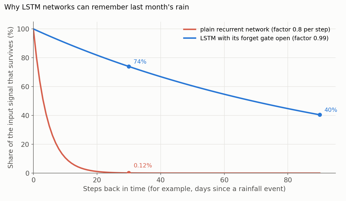
Figure 1. Why LSTM networks can remember. If a signal is multiplied by a constant factor at every step, a plain recurrent network with an effective factor of 0.8 keeps almost nothing of an input from 30 steps back, while an LSTM cell whose forget gate stays open (factor 0.99) keeps most of it. The factors are chosen for illustration; in real networks they are learned and change over time. Figure by Daeha Kim; illustrative, no data.
For hydrologists, Figure 1 is more than an abstraction. A catchment’s response today depends on rain that fell weeks ago and on snow that fell months ago. A model that forgets after a few days cannot represent that memory; one with a learned, gated store can, which is why LSTM networks later became the workhorse of machine learning in hydrology.
Deep learning returns (2006–2012)
The revival began with a trick for training networks with many layers. Geoffrey Hinton and colleagues showed that a deep network could be trained one layer at a time, each layer learning to represent the output of the layer below, and then fine-tuned as a whole (Hinton et al. 2006; Hinton & Salakhutdinov 2006). The word “deep,” meaning many layers, entered the field’s vocabulary.
Two other ingredients arrived at the same time. The first was computing power from an unexpected source: graphics processing units (GPUs), built to render video games, turned out to be very good at the matrix arithmetic that neural networks need, and training on them was dramatically faster than on ordinary processors (Raina et al. 2009). The second was data. Fei-Fei Li and colleagues built ImageNet, a database of millions of photographs labeled by thousands of crowd workers according to a hierarchy of object categories (Deng et al. 2009). From 2010 its annual challenge asked programs to classify images into 1,000 categories after training on about 1.2 million labeled examples (Russakovsky et al. 2015).
Not every headline of the period came from deep learning. In 2011 IBM’s Watson won the quiz show Jeopardy! against two of its strongest champions, using a large pipeline of many different language-processing and retrieval methods rather than a single learned network (Ferrucci et al. 2010). But in speech recognition, four research groups reported in 2012 that deep neural networks had overtaken the methods that had dominated the field for decades (Hinton et al. 2012).
2012: the year the benchmark broke
The turning point came at the 2012 ImageNet challenge. A deep convolutional network built by Alex Krizhevsky, Ilya Sutskever and Hinton, trained for several days on two consumer graphics cards, cut the top-5 error (the share of images whose correct label was not among the program’s five best guesses) to 16.4%, about ten percentage points ahead of the next-best entry (Krizhevsky et al. 2017; Russakovsky et al. 2015). The previous year’s winner had scored 25.8%. Within two years almost every competitive entry was a deep network.
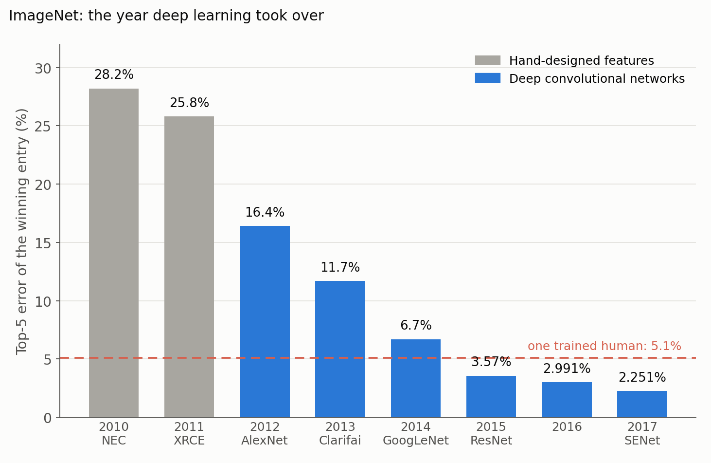
Figure 2. Top-5 classification error of the winning entry in the ImageNet challenge, 2010–2017. Gray bars are methods based on hand-designed image features; blue bars are deep convolutional networks. The dashed line is the error of one trained human annotator on 1,500 test images; a second annotator with less training scored 12.0%. Figure by Daeha Kim, drawn from numbers reported in Russakovsky et al. (2015), He et al. (2016) and Hu et al. (2018).
The error kept falling. In 2015 a residual network, which adds shortcut connections so that a network can be more than a hundred layers deep and still train, reached 3.57% (He et al. 2016). That was below the 5.1% measured for one carefully trained human annotator, and the result was widely reported as “superhuman.” The more careful statement is narrower: on this benchmark, with these 1,000 categories, the machine made fewer top-5 errors than one expert who had practiced for the task. A second annotator with less practice scored 12.0% (Russakovsky et al. 2015). By 2017 the winning error was 2.25%, and the challenge ended (Hu et al. 2018). The pattern will look familiar from my post on vibe coding: a public benchmark drives rapid progress, and then the meaning of the score becomes the hard question.
Learning by playing (2013–2017)
Deep networks next learned to act. DeepMind combined a convolutional network with reinforcement learning, in which a program learns from rewards rather than labeled examples, and trained a single system to play 49 Atari video games from the screen pixels and the score alone, reaching a level comparable to a professional games tester (Mnih et al. 2015).
Then came Go, a game with far too many possible positions for Deep Blue’s brute-force search. AlphaGo used two deep networks, one to suggest promising moves and one to evaluate positions, trained first on records of human games and then by playing against itself, and combined them with tree search. It beat the European champion Fan Hui 5–0 (Silver et al. 2016), and in March 2016, in Seoul, it beat Lee Sedol, one of the strongest players of the previous decade, by four games to one. For many people in Korea that match, more than any paper, marked the moment AI became real. A year later AlphaGo Zero learned the game from the rules alone, with no human games at all, and beat the version that had defeated Lee Sedol by 100 games to 0 (Silver et al. 2017).
The contrast with Part 1 is the clearest summary of these twenty years. Deep Blue’s strength came from its builders’ knowledge of chess, encoded by hand. AlphaGo Zero’s came from the rules of the game and an enormous amount of self-play.
Language: from word vectors to attention (2013–2017)
Language was harder, because meaning depends on context. A first step was to represent each word as a list of numbers learned from the contexts it appears in, so that words with similar meanings end up close together; word2vec made this fast enough to train on billions of words (Mikolov et al. 2013). Next, sequence-to-sequence models used one LSTM to read a sentence and another to write its translation (Sutskever et al. 2014). Their weakness was that the whole input sentence had to be squeezed into a single fixed-length summary. The fix, called attention, let the translating network look back at every word of the input and decide which ones mattered for the word it was writing (Bahdanau et al. 2015). In the same period, generative adversarial networks showed that two networks trained against each other could produce convincing new images (Goodfellow et al. 2014).
By 2015 the change was large enough for LeCun, Yoshua Bengio and Hinton to summarize it in a review in Nature (LeCun et al. 2015); the three later shared the 2018 Turing Award. And in June 2017 a team at Google proposed a translation model that dropped recurrence altogether and was built from attention alone. Because it processed all the words of a sentence at once rather than one at a time, it could be trained far more efficiently on GPUs. They called it the Transformer (Vaswani et al. 2017). Part 3 begins with what happened when people made it very large.
Hydrology catches up
Our field followed with a short delay. In 2018 Frederik Kratzert and colleagues showed that LSTM networks trained on daily meteorological data could simulate streamflow in hundreds of catchments in the United States with skill comparable to a well-established conceptual model, and that the network’s internal memory cells behaved in some ways like the snow and soil storages of a conceptual model (Kratzert et al. 2018). In the same year, Chaopeng Shen reviewed what deep learning could offer water resources science (Shen 2018). The question Hsu, Gupta and Sorooshian had raised in 1995, whether a network that predicts well can also teach us something, had come back in a stronger form.
What changed in twenty years
Three ingredients arrived together. The ideas behind deep learning (multilayer networks, backpropagation, convolution, LSTM) were mostly older than 2006. What changed was the arrival of large labeled data sets and cheap parallel computing, which finally made those ideas work at scale. Part 1 showed promises running ahead of data and computing power; Part 2 shows what happened when they caught up.
Learning replaced hand design, even for the inputs. Before 2012, image recognition relied on features designed by experts. After 2012, networks learned their own features from raw pixels. AlphaGo Zero took the same step for game knowledge. The trend is still running.
Benchmarks became the engine of progress, and the arguments moved with them. ImageNet focused a whole field on one number. It also showed how easily a narrow score can be read as a broad claim.
Bottom line
- From the late 1990s, statistical learning methods replaced hand-written rules; Breiman’s “two cultures” named the split between explaining and predicting that hydrology knows well.
- Two older ideas, convolutional networks and LSTM memory, became the building blocks of the deep-learning era.
- Deep learning returned around 2006 and took over after 2012, when a GPU-trained network cut the ImageNet error by about ten percentage points.
- AlphaGo (2016) and AlphaGo Zero (2017) showed that learning and self-play could beat the hand-built knowledge that powered Deep Blue.
- Attention (2014) and the Transformer (2017) set the stage for the large language models of Part 3; hydrology adopted LSTM networks from 2018.
Questions to think about
- Breiman described two cultures of statistical modeling. Which one does your own research belong to, and what would you gain from the other?
- Why does a model of daily streamflow need memory? List the processes in a catchment that make today’s flow depend on last month’s weather.
- A network beat one trained human on ImageNet in 2015. What would it take for you to call a hydrological model “better than an expert hydrologist”?
한 줄 요약 (Korean summary). 인공지능 역사 연재의 두 번째 편으로, 딥 블루 이후 트랜스포머가 나오기까지(1997–2017)를 다룬다. 1990년대 후반부터는 규칙을 직접 쓰는 대신 데이터로부터 학습하는 통계적 방법(서포트 벡터 머신, 랜덤 포레스트)이 주류가 되었고, 브라이먼은 자료가 생성되는 과정을 모형으로 가정하는 문화와 예측력만으로 모형을 평가하는 문화를 “두 문화”로 구분했다. 이는 수문학의 개념적 모형과 자료 기반 모형 사이의 긴장과 같다. 이 시기 합성곱 신경망과 LSTM(게이트로 무엇을 기억하고 잊을지 정하는 순환 신경망)이라는 두 아이디어가 나중의 핵심 부품이 되었다. 2006년 무렵 층별 사전학습으로 깊은 신경망이 되살아났고, 게임용 그래픽 카드(GPU)의 계산 능력과 ImageNet이라는 대규모 라벨 데이터가 더해지면서, 2012년 GPU로 학습한 합성곱 신경망이 ImageNet 오류율을 16.4%로 낮춰 2위보다 약 10%p 앞섰다. 2015년 ResNet은 3.57%로 훈련된 한 사람의 5.1%보다 낮아졌지만, 이는 특정 벤치마크에서 한 사람과 비교한 결과일 뿐이다. 이어 딥마인드의 강화학습은 화면 픽셀만으로 아타리 게임 49종을 익혔고, 알파고는 2016년 3월 서울에서 이세돌 9단을 4승 1패로 이겼으며, 이듬해 알파고 제로는 사람의 기보 없이 규칙과 자기 대국만으로 이전 알파고를 100대 0으로 이겼다. 언어 분야에서는 단어 벡터, 시퀀스-투-시퀀스 번역, 어텐션을 거쳐 2017년 어텐션만으로 이루어진 트랜스포머가 나왔다. 수문학도 2018년 LSTM이 미국의 수백 개 유역에서 기존 개념적 모형에 견줄 만한 유출 모의 성능을 보이면서 본격적으로 딥러닝을 받아들였다. 이 20년의 핵심은 오래된 아이디어에 대규모 데이터와 값싼 병렬 계산이 더해진 것, 그리고 사람이 설계하던 특징과 지식을 학습이 대신하게 된 것이다.
References
Bahdanau, D., Cho, K., & Bengio, Y. (2015). Neural machine translation by jointly learning to align and translate. In International Conference on Learning Representations (ICLR 2015). arXiv:1409.0473. https://doi.org/10.48550/arXiv.1409.0473
Breiman, L. (2001a). Random forests. Machine Learning, 45(1), 5–32. https://doi.org/10.1023/A:1010933404324
Breiman, L. (2001b). Statistical modeling: The two cultures. Statistical Science, 16(3), 199–231. https://doi.org/10.1214/ss/1009213726
Cortes, C., & Vapnik, V. (1995). Support-vector networks. Machine Learning, 20(3), 273–297. https://doi.org/10.1007/BF00994018
Deng, J., Dong, W., Socher, R., Li, L.-J., Li, K., & Fei-Fei, L. (2009). ImageNet: A large-scale hierarchical image database. In 2009 IEEE Conference on Computer Vision and Pattern Recognition, 248–255. https://doi.org/10.1109/CVPR.2009.5206848
Ferrucci, D., Brown, E., Chu-Carroll, J., Fan, J., Gondek, D., Kalyanpur, A. A., et al. (2010). Building Watson: An overview of the DeepQA project. AI Magazine, 31(3), 59–79. https://doi.org/10.1609/aimag.v31i3.2303
Goodfellow, I. J., Pouget-Abadie, J., Mirza, M., Xu, B., Warde-Farley, D., Ozair, S., Courville, A., & Bengio, Y. (2014). Generative adversarial networks. arXiv:1406.2661. https://doi.org/10.48550/arXiv.1406.2661
He, K., Zhang, X., Ren, S., & Sun, J. (2016). Deep residual learning for image recognition. In 2016 IEEE Conference on Computer Vision and Pattern Recognition, 770–778. https://doi.org/10.1109/CVPR.2016.90
Hinton, G. E., Osindero, S., & Teh, Y.-W. (2006). A fast learning algorithm for deep belief nets. Neural Computation, 18(7), 1527–1554. https://doi.org/10.1162/neco.2006.18.7.1527
Hinton, G. E., & Salakhutdinov, R. R. (2006). Reducing the dimensionality of data with neural networks. Science, 313(5786), 504–507. https://doi.org/10.1126/science.1127647
Hinton, G., Deng, L., Yu, D., Dahl, G. E., Mohamed, A.-r., Jaitly, N., et al. (2012). Deep neural networks for acoustic modeling in speech recognition: The shared views of four research groups. IEEE Signal Processing Magazine, 29(6), 82–97. https://doi.org/10.1109/MSP.2012.2205597
Hochreiter, S., & Schmidhuber, J. (1997). Long short-term memory. Neural Computation, 9(8), 1735–1780. https://doi.org/10.1162/neco.1997.9.8.1735
Hu, J., Shen, L., & Sun, G. (2018). Squeeze-and-excitation networks. In 2018 IEEE/CVF Conference on Computer Vision and Pattern Recognition, 7132–7141. https://doi.org/10.1109/CVPR.2018.00745
Kratzert, F., Klotz, D., Brenner, C., Schulz, K., & Herrnegger, M. (2018). Rainfall–runoff modelling using Long Short-Term Memory (LSTM) networks. Hydrology and Earth System Sciences, 22(11), 6005–6022. https://doi.org/10.5194/hess-22-6005-2018
Krizhevsky, A., Sutskever, I., & Hinton, G. E. (2017). ImageNet classification with deep convolutional neural networks. Communications of the ACM, 60(6), 84–90 (first presented at NeurIPS 2012). https://doi.org/10.1145/3065386
LeCun, Y., Bengio, Y., & Hinton, G. (2015). Deep learning. Nature, 521(7553), 436–444. https://doi.org/10.1038/nature14539
LeCun, Y., Bottou, L., Bengio, Y., & Haffner, P. (1998). Gradient-based learning applied to document recognition. Proceedings of the IEEE, 86(11), 2278–2324. https://doi.org/10.1109/5.726791
Mikolov, T., Chen, K., Corrado, G., & Dean, J. (2013). Efficient estimation of word representations in vector space. arXiv:1301.3781. https://doi.org/10.48550/arXiv.1301.3781
Mnih, V., Kavukcuoglu, K., Silver, D., Rusu, A. A., Veness, J., Bellemare, M. G., et al. (2015). Human-level control through deep reinforcement learning. Nature, 518(7540), 529–533. https://doi.org/10.1038/nature14236
Raina, R., Madhavan, A., & Ng, A. Y. (2009). Large-scale deep unsupervised learning using graphics processors. In Proceedings of the 26th Annual International Conference on Machine Learning, 873–880. https://doi.org/10.1145/1553374.1553486
Russakovsky, O., Deng, J., Su, H., Krause, J., Satheesh, S., Ma, S., et al. (2015). ImageNet Large Scale Visual Recognition Challenge. International Journal of Computer Vision, 115(3), 211–252. https://doi.org/10.1007/s11263-015-0816-y
Shen, C. (2018). A transdisciplinary review of deep learning research and its relevance for water resources scientists. Water Resources Research, 54(11), 8558–8593. https://doi.org/10.1029/2018WR022643
Silver, D., Huang, A., Maddison, C. J., Guez, A., Sifre, L., van den Driessche, G., et al. (2016). Mastering the game of Go with deep neural networks and tree search. Nature, 529(7587), 484–489. https://doi.org/10.1038/nature16961
Silver, D., Schrittwieser, J., Simonyan, K., Antonoglou, I., Huang, A., Guez, A., et al. (2017). Mastering the game of Go without human knowledge. Nature, 550(7676), 354–359. https://doi.org/10.1038/nature24270
Sutskever, I., Vinyals, O., & Le, Q. V. (2014). Sequence to sequence learning with neural networks. arXiv:1409.3215. https://doi.org/10.48550/arXiv.1409.3215
Vaswani, A., Shazeer, N., Parmar, N., Uszkoreit, J., Jones, L., Gomez, A. N., Kaiser, Ł., & Polosukhin, I. (2017). Attention is all you need. arXiv:1706.03762. https://doi.org/10.48550/arXiv.1706.03762
Both figures are original. The Python scripts that produce them are available on GitHub: Figure 1 and Figure 2.